This vignette shows how to use the package to emulate a feed-forward system of three synthetic computer models.
Construct a synthetic system
We consider the following synthetic system

that involves three models defined by:
# Model 1
f1 <- function(x) {
  (sin(7.5*x)+1)/2
}
# Model 2
f2 <- function(x) {
  2/3*sin(2*(2*x - 1))+4/3*exp(-30*(2*(2*x-1))^2)-1/3
}
# Model 3
f3 <- function(x) {
  x[1]*x[2]^2
}
# Linked Model
f123 <- function(x) {
  f3(c(f1(x),f2(f1(x))))
}
We then specify a seed with set_seed() from the package
for reproducibility
set_seed(999)and generate 10 training data points for Model 1 and 15 training data points for Model 2 and 3:
Emulation of Model 1
We construct and train a GP emulator with Matérn-2.5 kernel with ID
gp1:
m1 <- gp(X1, Y1, name = "matern2.5", id = "gp1")## Auto-generating a GP structure ... done
## Initializing the GP emulator ... done
## Training the GP emulator ... doneWe now validate the trained GP emulator by plot() by LOO
(alternatively, one can first use validate() to store the
LOO results before plotting with plot()):
plot(m1)## Validating and computing ... done
## Post-processing LOO results ... done
## Plotting ... done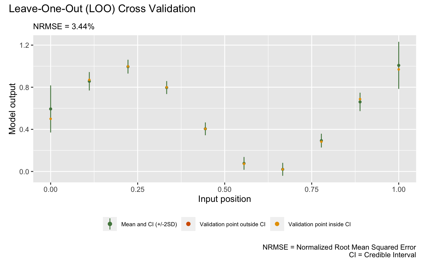
Emulation of Model 2
We construct a two-layered DGP emulator with Matérn-2.5 kernels to emulate Model 2:
m2 <- dgp(X2, Y2, depth = 2, name = "matern2.5")## Auto-generating a 2-layered DGP structure ... done
## Initializing the DGP emulator ... done
## Training the DGP emulator:
## Iteration 500: Layer 2: 100%|██████████| 500/500 [00:01<00:00, 264.72it/s]
## Imputing ... doneand set its ID to gp2 using the set_id()
function:
m2 <- set_id(m2, "gp2")The following plot visualizes the LOO of the trained DGP emulator
m2:
plot(m2)Validating and computing ... done
Post-processing LOO results ... done
Plotting ... done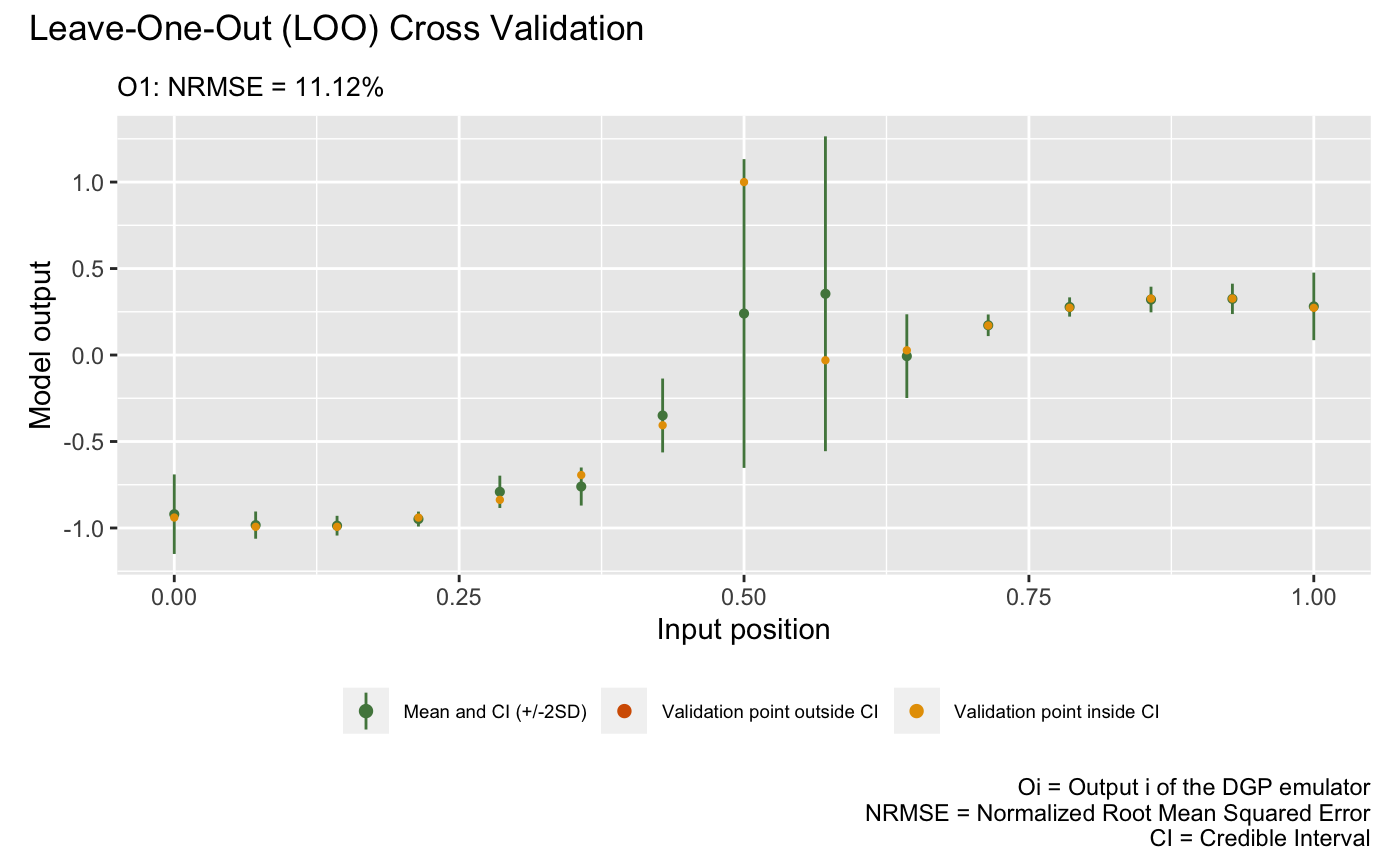
Emulation of Model 3
We now construct a three-layered DGP emulator with Matérn-2.5 kernels to emulate Model 3:
m3 <- dgp(X3, Y3, depth = 3, name = "matern2.5", id = "gp3" )## Auto-generating a 3-layered DGP structure ... done
## Initializing the DGP emulator ... done
## Training the DGP emulator:
## Iteration 500: Layer 3: 100%|██████████| 500/500 [00:04<00:00, 104.80it/s]
## Imputing ... doneThe following plot visualizes the LOO of the trained DGP emulator
m3:
plot(m3)Validating and computing ... done
Post-processing LOO results ... done
Plotting ... done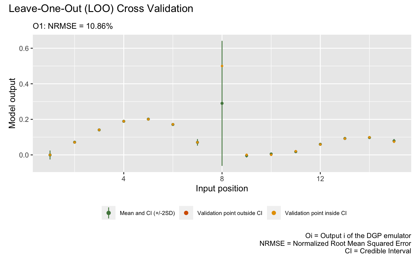
Emulation of Linked Model
With the GP emulator m1 (for Model 1), the DGP emulator
m2 (for Model 2), and the DGP emulator m3 (for
Model 3) at hand, we are now ready to build the linked emulator by first
defining a data frame struc:
struc <- data.frame(From_Emulator = c("Global", "gp1", "gp1", "gp2"),
                    To_Emulator = c("gp1", "gp2", "gp3", "gp3"),
                    From_Output = c(1, 1, 1, 1),
                    To_Input = c(1, 1, 1, 2))
struc
## From_Emulator To_Emulator From_Output To_Input
## 1 Global gp1 1 1
## 2 gp1 gp2 1 1
## 3 gp1 gp3 1 1
## 4 gp2 gp3 1 2The struc data frame above defines the feed-forward
connection structure between the three emulators in the linked system.
Each row represents a one-to-one connection between an output dimension
(From_Output) of a source emulator
(From_Emulator) and an input dimension
(To_Input) of a target emulator
(To_Emulator).
For example: - The first row specifies that the global input (denoted
by Global)’s first dimension (column) is connected to the
first input dimension of emulator gp1. - The second row
indicates that the first output dimension of emulator gp1
is connected to the first input dimension of emulator
gp2.
Finally, we can pass struc and a list of the three
trained emulators to lgp() to create the linked emulator.
The order of the emulators in the list does not matter:
emulators <- list(m1, m2, m3)Before activating the linked emulator for prediction, it’s good practice to first inspect the structure of the emulator:
m_link <- lgp(struc, emulators, activate = FALSE)Processing emulators ... done
Linking and synchronizing emulators ... doneand visually check the relationships between emulators by applying
summary() to m_link:
summary(m_link)If everything looks correct, we can then activate the linked emulator for prediction:
m_link <- lgp(struc, emulators, activate = TRUE)Processing emulators ... done
Linking and synchronizing emulators ... done
Activating the linked emulator ... doneFor comparison, we construct a GP emulator for the whole system by generating 15 training data points from Model 1 and Model 2:
X_gp <- seq(0, 1, length = 15)
Y_gp <- sapply(X_gp, f123)
m_gp <- gp(X_gp, Y_gp, name = 'matern2.5')
## Auto-generating a GP structure ... done
## Initializing the GP emulator ... done
## Training the GP emulator ... doneFinally, we validate both the GP emulator and the linked emulator at 300 testing data points over :
# Testing input
test_x <- seq(0, 1, length = 300)
# Testing output
test_y <- sapply(test_x, f123)
# Validate GP emulator
m_gp <- validate(m_gp, x_test = test_x, y_test = test_y, verb = F)
# Validate linked emulator
m_link <- validate(m_link, x_test = test_x, y_test = test_y, verb = F)
and plot them to compare their performance:
# GP emulator
plot(m_gp, x_test = test_x, y_test = test_y, type = 'line', verb = F) +
  plot_annotation(title = 'GP Emulator', theme = theme(plot.title = element_text(hjust = 0.5)))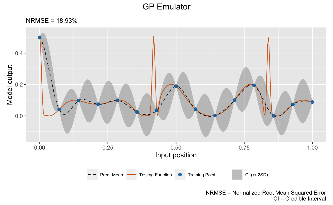
# Linked emulator
plot(m_link, x_test = test_x, y_test = test_y, type = 'line', verb = F) +
  plot_annotation(title = 'Linked Emulator', theme = theme(plot.title = element_text(hjust = 0.5)))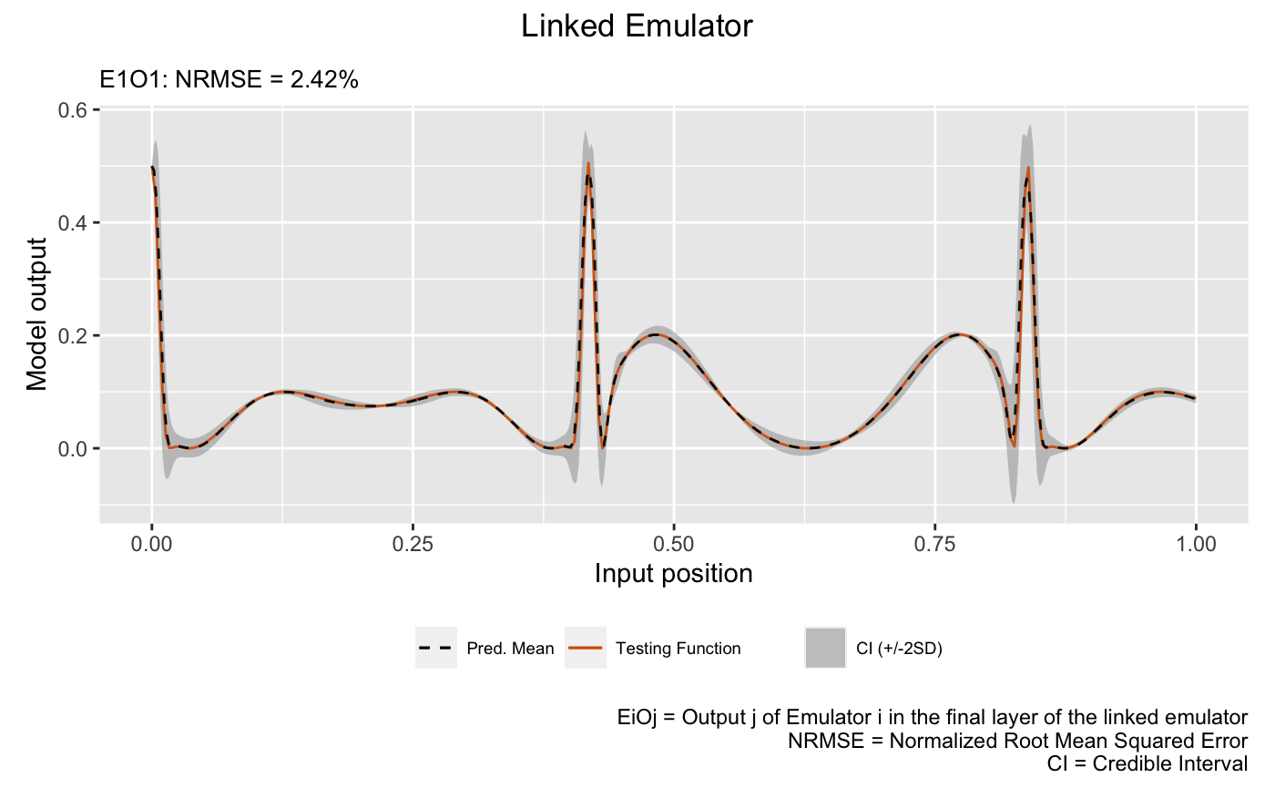
We see that the linked emulator outperforms the GP emulator with significantly better mean prediction and uncertainty quantification.
In real-life applications, we are rarely able to generate this many testing data points from the underlying computer simulators to evaluate the emulators over the whole input space. However, we are still able to retain some available realizations from the computer simulators for validation. Say we were able to afford 20 runs of the above linked computer system:
# OOS testing input
test_x_oos <- sample(seq(0, 1, length = 300), 20)
# OOS testing output
test_y_oos <- sapply(test_x_oos, f123)
Then, we can conduct OOS validation for the GP emulator:
plot(m_gp, test_x_oos, test_y_oos, style = 2)## Validating and computing ... done
## Post-processing OOS results ... done
## Plotting ... done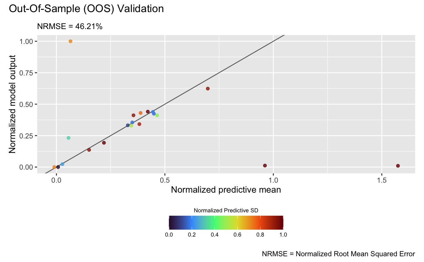
and the linked emulator:
plot(m_link, test_x_oos, test_y_oos, style = 2)## Validating and computing ... done
## Post-processing OOS results ... done
## Plotting ... done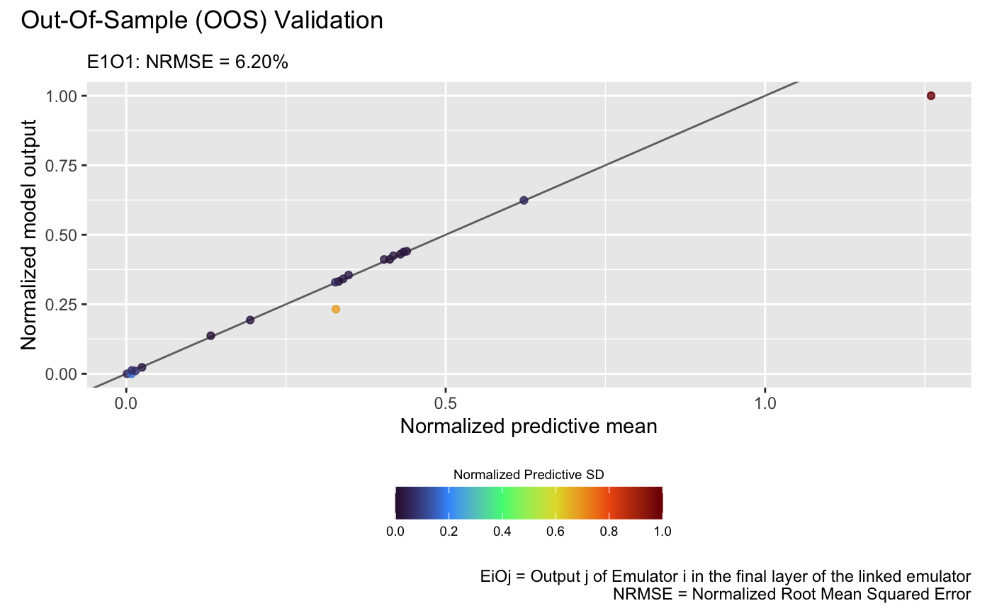
which show that the linked emulator outperforms the GP emulator with significantly better predictive accuracy and lower NRMSE.
