A Quick Guide to dgpsi

dgpsi provides a flexible toolbox for Gaussian process (GP), deep Gaussian process (DGP) and linked (D)GP emulations. In this guide, we show how to use the package to emulate a step function with a three-layered DGP structure. There are other examples showing the functionality of the package in Articles on the package website, and how to customize a DGP structure. A comprehensive reference of available functions is documented in Reference section of the package website.

Load the package

library(dgpsi)

Set up the step function

dgpsi provides a function init_py() that helps us set up, initialize, re-install, or uninstall the underlying Python environment. We could run init_py() every time after dgpsi is loaded to manually initiate the Python environment. Alternatively, we could activate the Python environment by simply executing a function from dgpsi. For example, the Python environment will be automatically loaded after we run set_seed() from the package to specify a seed for the reproducibility:

set_seed(9999)

We then define the step function:

f <- function(x) {
  if (x < 0.5) return(-1)
  if (x >= 0.5) return(1)
}

and generate ten training data points:

X <- seq(0, 1, length = 10)
Y <- sapply(X, f)

Training

We now build and train a DGP emulator with three layers:

m <- dgp(X, Y, depth = 3)

## Auto-generating a 3-layered DGP structure ... done
## Initializing the DGP emulator ... done
## Training the DGP emulator: 
## Iteration 500: Layer 3: 100%|██████████| 500/500 [00:03<00:00, 148.10it/s]
## Imputing ... done

The progress bar displayed shows how long it takes to finish the training. We are able to switch off the progress bar and the trace information by setting verb = FALSE. Note that if we want to train the DGP emulator m for additional iterations, we can simply do m <- continue(m) instead of rebuilding the DGP emulator.

The trained DGP emulator can be visualized using the summary() function:

summary(m)

The visualization also gives key information about the trained DGP emulator. Note that in the auto-generated emulator we have nugget terms fixed to 1e-6 for all GP nodes because we are emulating a deterministic step function (i.e., we would like our emulator to interpolate training data points). The prior scales (i.e., variances) for GP nodes in the first and second layers are fixed to 1.0 while that for the GP node in the final layer is estimated due to its attachment to the output. For further information on how to change the default settings to construct and train a DGP emulator, see ?dgp.

At this point, you could use write() to save the emulator m to a local file and then load it using read() when you would like to make predictions from the emulator, e.g., on another laptop that also has the package installed.

Validation

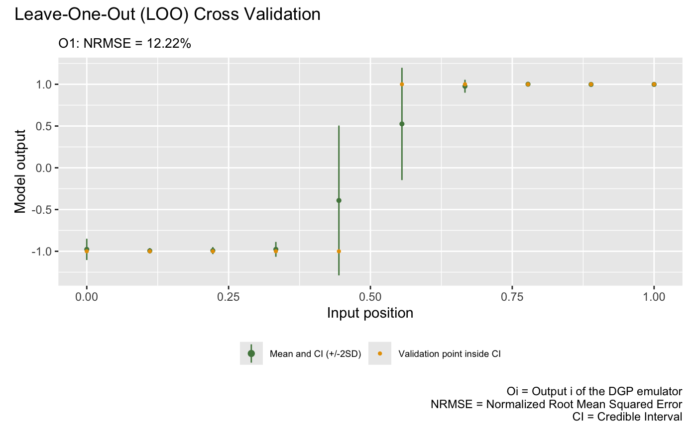
After we have the emulator, we can validate it by drawing the validation plots. There are two types of validation plots provided by the package. The first one is the Leave-One-Out (LOO) cross validation plot:

plot(m)

## Validating and computing ... done
## Post-processing LOO results ... done
## Plotting ... done

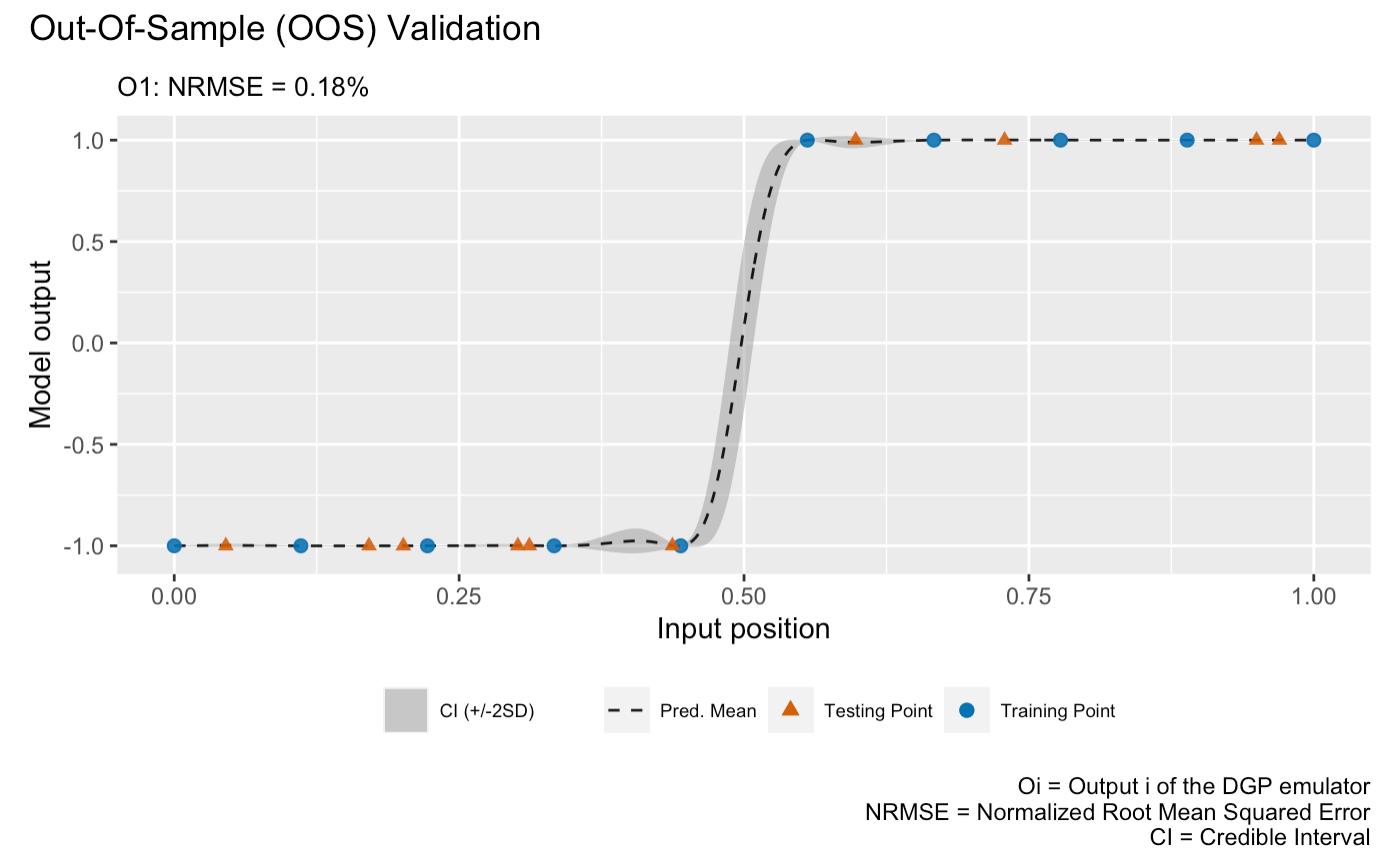
The second validation plot is the Out-Of-Sample (OOS) validation plot that requires an out-of-sample testing data set. Here we generate an OOS data set that contains 10 testing data points

oos_x <- sample(seq(0, 1, length = 200), 10)
oos_y <- sapply(oos_x, f)

for the validation:

plot(m,oos_x,oos_y)

## Validating and computing ... done
## Post-processing OOS results ... done
## Plotting ... done

Prediction

Once the validation is done, we can make predictions from the DGP emulator. We generate 200 data points from the step function over $[0,1]$

test_x <- seq(0, 1, length = 200)
test_y <- sapply(test_x, f)

for predictions:

m <- predict(m, x = test_x)

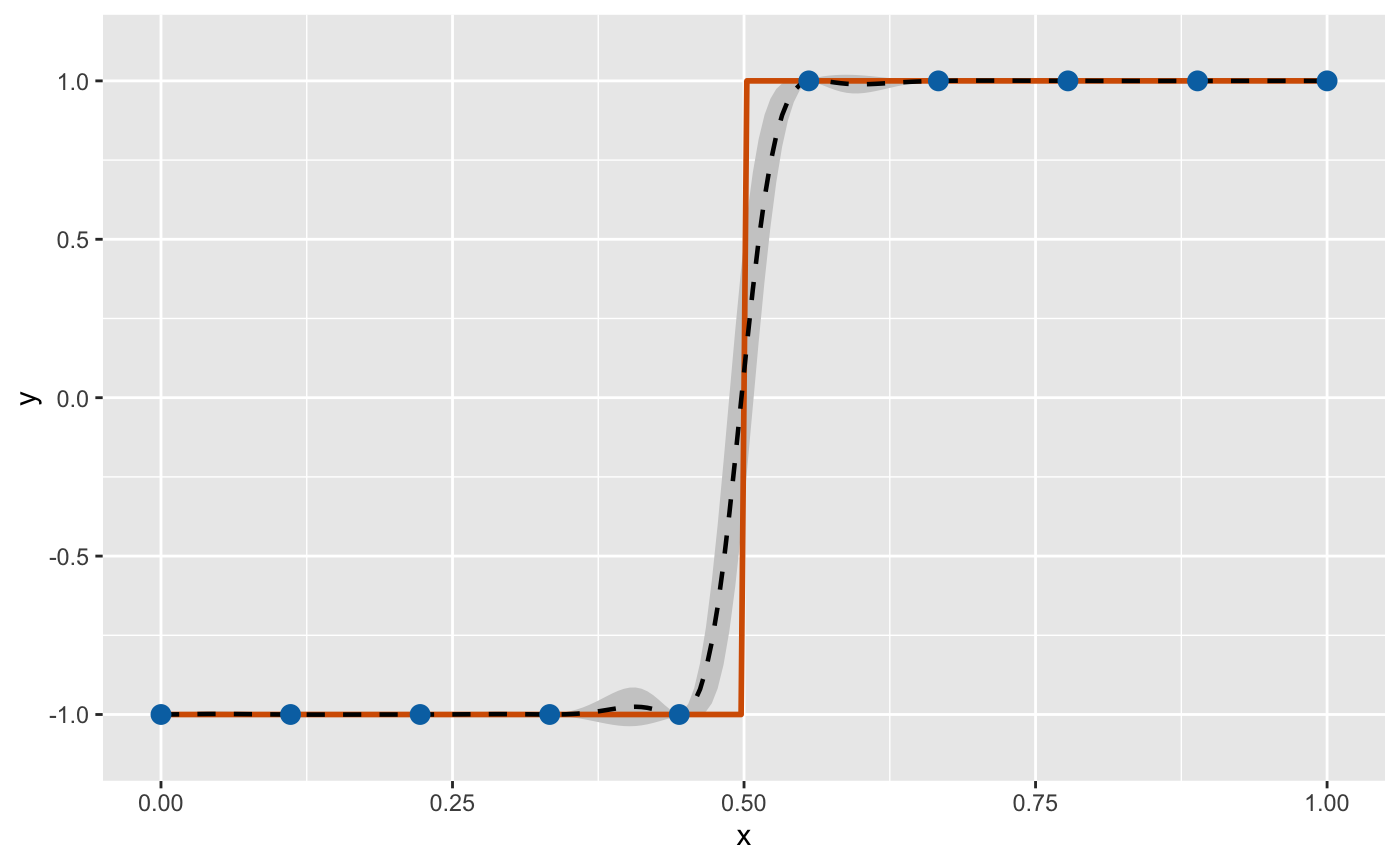
The predict() function returns an updated DGP emulator m that contains a slot named results that gives the posterior predictive means and variances at testing positions. We can extract these information and plot the emulation results to check the predictive performance of our constructed DGP emulator:

mu <- m$results$mean # extract the predictive means 
sd <- sqrt(m$results$var) # extract the predictive variance and compute the predictive standard deviations
# compute predictive bounds which are two predictive standard deviations above and below the predictive means
up <- mu + 2*sd 
lo <- mu - 2*sd

plot(test_x, mu, type = 'l', lty = 2, lwd = 1.5, col = 'black', xlab = 'x', cex.axis = 1.3, cex.lab = 1.3, ylab = 'y', ylim = c(-1.5,1.5))  # predictive means 
polygon(c(test_x, rev(test_x)), c(up,rev(lo)), col = 'grey80', border = F) # credible interval
lines(test_x, test_y, type = 'l', col = "#D55E00", lwd = 2) # Underlying truth
lines(test_x, mu, type = 'l', lty = 2, lwd = 1.5, col = 'black')
lines(X, Y, type = 'p', pch = 16, cex = 1, col = "#0072B2") # Training data points