This vignette gives a demonstration of the package on classifying the popular iris data set (Anderson 1935).
Load packages and data
We start by loading required packages,
We now load the iris data set,
data(iris)and re-scale its four input variables to .
Before building a classifier, we set a seed with
set_seed() from the package for reproducibility
set_seed(9999)and split the data into training and testing:
Construct and train a DGP classifier
We consider a three-layer DGP classifier using Matérn-2.5 kernels:
m_dgp <- dgp(X_train, Y_train, depth = 3, name = 'matern2.5', likelihood = "Categorical")## Auto-generating a 3-layered DGP structure ... done
## Initializing the DGP emulator ... done
## Training the DGP emulator:
## Iteration 500: Layer 3: 100%|██████████| 500/500 [00:52<00:00, 9.44it/s]
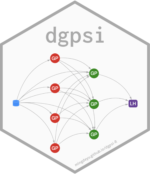
## Imputing ... doneVisualizing the DGP object helps to clarify the layered structure for non-Gaussian (in this case categorical) likelihoods.
summary(m_dgp)After the global inputs, the 3-layered DGP is comprised of 2 hidden layers containing GPs, and a “likelihood layer” that transforms each of the preceding GP nodes to one of the parameters required by the likelihood function. In this example, we have 3 possible categories and we use a softmax link function, so there are 3 parameters to set and the second layer has 3 GP nodes, one for each of them.
Validation
We are now ready to validate the classifier via
validate() at 30 out-of-sample testing positions:
m_dgp <- validate(m_dgp, X_test, Y_test)## Initializing the OOS ... done
## Calculating the OOS ... done
## Saving results to the slot 'oos' in the dgp object ... doneFinally, we visualize the OOS validation for the classifier:
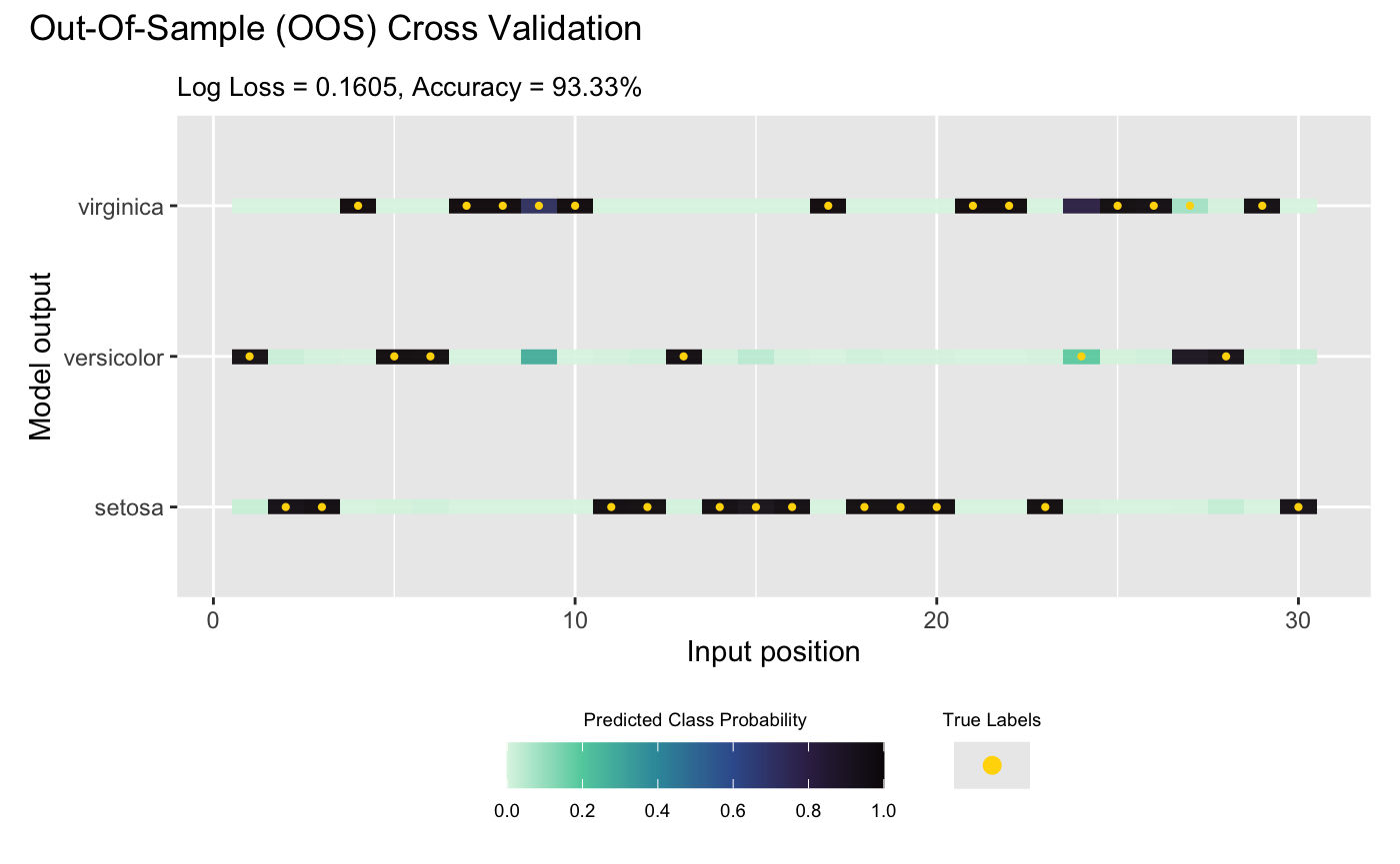
plot(m_dgp, X_test, Y_test)## Validating and computing ... done
## Post-processing OOS results ... done
## Plotting ... done
By default, plot() displays true labels against
predicted label proportions at each input position. Alternatively,
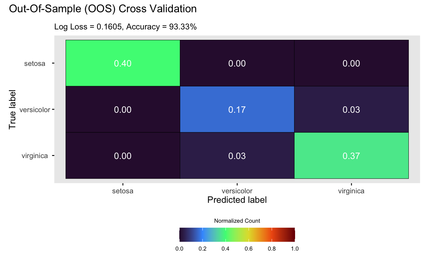
setting style = 2 in plot() generates a
confusion matrix:
plot(m_dgp, X_test, Y_test, style = 2)## Validating and computing ... done
## Post-processing OOS results ... done
## Plotting ... done
